What does it mean for a model to “scale”? (Part 9)
(This post is part of a series on working with data from start to finish.)
In my examination of model accuracy, I alluded to the fact that traditional statistics focuses on inference while machine learning focuses on prediction.
Model scalability relates to the latter: as we observe new data, does the model make better or worse predictions over time?
If instead we focus solely on inference, we find it is not particularly difficult to infer a model that fits historically observed data with 100% accuracy. For example, imagine a set of colored marbles rolling out from an opening in the wall. The first five marbles are red, blue, green, red, blue (in that order).
| sequence | color |
|---|---|
| 1 | red |
| 2 | blue |
| 3 | green |
| 4 | red |
| 5 | blue |
Given this data, you could easily develop a model that perfectly retrodicts each observation. In natural language, one such model could be: “When observing the first marble, assign red; the second blue; the third green; the fourth red; and the fifth green”. This model takes the marble sequence number as input and assigns color as output.
Expressed as a statistical model, this model would be:
yi = β0 + β1xi,1 + β2xi,2 + β3xi,3 + β4xi,4 + β5xi,5 + ε,
where β equals 0 when red, 1 when blue, and 2 when green.
Here, each independent variable represents a boolean flag for the marble sequence number. When the sequence number is 2, xi,2 equals 1 (true) and all other parameters equal 0 (false). As yi is observed to be 1 (blue), β2 must be 1. The same holds for sequence number 3: xi,3 equals 1 while other variables equal 0, and when yi is observed to be 2 (green), β3 must be 2.
This model explains the observed data with 100% accuracy. The error term, or random variation, equals 0.
Model accuracy versus model parsimony #
No matter the description language, one thing remains the same: adding more parameters to a model will improve model fit, but only at the expense of parsimony. This is known as “the inflation of R²”, the reason for which an adjusted R² (penalized for parameter count) is often used instead of the original R².
Contrary to one might expect, an R² of 100% is not ideal. It suggests the model overfits the original data. It hugs each historical data point too closely, rendering the model unable to generalize well to new, unseen data.
For example, what will this model predict the sixth marble’s color to be? It has no prediction (or null), which we already know cannot be the correct answer. After observing the sixth marble’s color, the model’s accuracy would fall to 5/6, or 83%.
Now imagine we conceived of a more parsimonious model. In natural language, it could be: “Given the marble sequence number, divide by three and take the remainder: when 0, assign green, when 1, red and when 2, blue.”
In a statistical model, this would conscript the rather pedestrian modulo operator (or mod(dividend, divisor)):
yi = β0 + β1mod(xi,1, 3) + ε,
where β equals 0 when green, 1 when red, and 2 when blue.
Here, the sole independent variable represents the marble sequence number. When the sequence number xi,1 is 2, then mod(2, 3) equals 2 (blue), which is the correct color of the second marble. When the sequence number xi,1 is 5, then mod(5, 3) again equals 2 (blue), which is the correct color of the fifth marble.
And what would the color of the sixth marble be? Compared to no prediction, this model would predict mod(6, 3) = 0, which is green.
Assuming the historical pattern holds, this considerably more parsimonious model (only 1 parameter!) would preserve its 100% accuracy even in the face of new, unseen data.
Let’s take another example. Imagine you are developing a standard operating procedure within your team for handling customer support inquiries. This model describes how an input (initial inquiry) flows through the system into a final, output state (resolved inquiry). There are likely many intricacies to this procedure which are idiosyncratic to your team: who handles the initial query, what systems to use, what steps are required to reach resolution, what the escalation process is.
If you were to force this same procedure upon another team, it would likely perform very poorly. This team might use different systems, have different team structure, or resolve inquiries differently. As a result, we would observe considerable error as the new team attempts to apply this inapposite standard operating procedure, which of course was never designed for them. Model accuracy as a whole - that is, across both teams and their corresponding sets of data - would fall.
In order for the model to scale across multiple teams, it would first have to be generalized: team-specific nuances would be replaced by team-agnostic ones. Components specific to each team would be removed from the model and replaced with fewer, more abstract components representing the commonalities between teams. Like our example with the marbles above, we would confect a more parsimonious operating model.
Metamodels which scale #
Although this integrated model would be different from the original model, it would contain commonalities from both the original team (i.e. original data) and the new team (i.e. new data). We might therefore call it a metamodel, or an abstracted model.
As it would contain fewer parameters specific to the original team, it would necessarily perform worse on the original data. However, when considering both sets of data (that is, the stacked data set), the model would perform better.
This suggests that as we remove and consolidate parameters from the original model, thereby transforming it into a more abstracted model, we correspondingly increase its accuracy when applied to new data. The metamodel reaches further. It scales farther.
When total accuracy increases as we increase parsimony, we might say that the derivative of accuracy with respect to parsimony, or dA/dP, is positive. This is our scaling coefficient S.
It is, however, entirely possible to construct a poor metamodel such that accuracy actually declines for both the original team and any new teams. It is not hard to imagine executive teams overhauling company workflows and systems in the name of “simplification” and “standardization”, which nevertheless have the ultimate effect of reducing efficiency for all teams. In such a case, the scaling coefficient dA/dP would be negative.
We can plot each scaling case as follows:
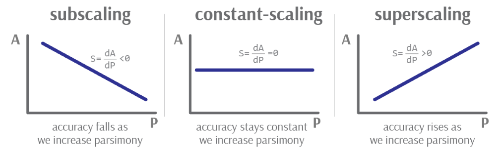
Image credit: Author’s own work
When the slope is negative, the model “subscales”: we reduce model accuracy as we make the model more parsimonious. When flat, the model “constant scales”: model accuracy does not vary as we make the model more parsimonious. And finally, when the slope is positive, the model “superscales”: model accuracy improves as we make the model more parsimonious.
Of course, we don’t only care about the sign of the scaling coefficient. We also care about its magnitude. A high positive scaling coefficient implies that relatively minor improvements in parsimony will considerably increase a model’s reach. On the other hand, a low scaling coefficient implies that the model model cannot be generalized broadly.
Is it possible to know in advance whether a model will scale positively or negatively?
No. A model’s scalability can only be evaluated against yet unseen data. A model that initially scales well may eventually scale poorly after a certain amount of data is reached. We might call this the model’s “scaling limit”, after which the model must be further refined and abstracted.