What makes a model "accurate"? (Part 7)
(This post is part of a series on working with data from start to finish.)
A model’s accuracy measures the degree of closeness between its modeled predictions about a system and the actual, measured observations emanating from that system. More specifically, as we vary one part of a system, we can make theoretical predictions about other parts of the system, and those predictions should align with what we actually observe. Immediately, from this definition, we see that a model has no concept of accuracy if (a) it does not make predictions or (b) if it does not measure observable outputs from a system.
Models can be expressed using a mathematical, algorithmic, schematic or natural language, likely among others as well. In each case, the model describes the relationships between parts in its given “description language”, which can be mathematical symbols, code, diagrams or words. The choice of description language is consequential: mathematics, for example, is precise and logical, while words are broad and generative. Mathematics then is conducive to deductive and rational thought, natural language to metaphorical and creative thought.
Different description languages can therefore aid or inhibit analysis of a system, an idea most famously popularized in the computer scientist Kenneth Iverson’s 1979 Notation as a Tool of Thought. Because of this, many description languages should be experimented with when attempting to model a new system.
Models in theory versus models in practice #
Most models are deterministic in nature, meaning that for any given input, we always get the same output. If you make a statement such as “tomorrow, it will rain”, this statement alone does not admit any randomness. Similarly, if you draw a schematic of how a TV operates, the diagram does not demonstrate how the TV sometimes works, but rather how it always, deterministically works. Most physical equations, such as the relationship between mass and acceleration (F=ma), also reflect deterministic relationships. Even quantum physics’ vaunted wave function, the Schrödinger equation, operates deterministically.
From where then does the notion of randomness arise?
Randomness originates not from the theoretical models themselves, but instead from the measurement of those models. Whenever we build models describing how the world works, we invariably observe outcomes that do not line up with what the model predicted. Because these models do not completely explain everything we actually end up observing, we are left with unexplained sources of variation, or “random error”. Put another way, deterministic models assume complete knowledge of a system, but real-world, measured data reveals incomplete knowledge of that system.
Randomness, therefore, is what remains after we explain everything we can. As we learn and explain more about how the world works, it will appear less and less random.
Accuracy as model fit #
When evaluating the accuracy of a model, we compare how well its predictions line up with real-world observations. We call this model fit: how well does the model fit the data? To calculate model fit, we invoke a statistical model. Importantly, and unlike strictly deterministic models, statistical models include a “random error” term to account for observed data the model does not completely explain.
Within a statistical model, the independent variables represent the systematic, deterministic portions of the model, while the error term represents the unsystematic, non-deterministic portion owing to measurement. If we were to make predictions from this model, we would only use the coefficients. If we were to then validate those predictions against real-world data, we would include the error term.
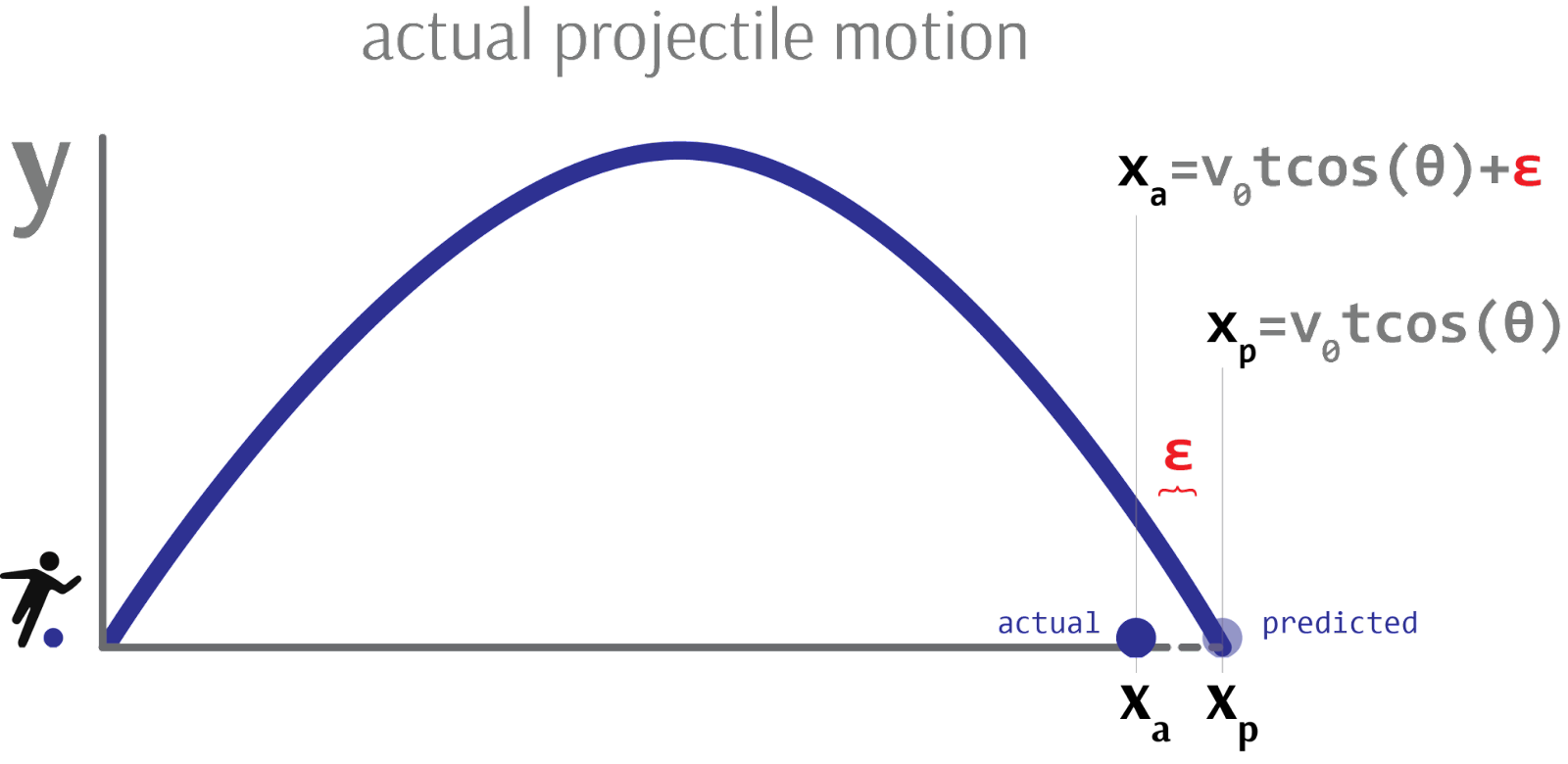 Image credit: Author’s own work
The inflation of R² #
As we add parts to our model - be it components in a schematic, terms in a physical equation, or conditionals in a piece of code - we are necessarily able to attribute more of what we observe to known parts of the model. That is, less of what we observe will be unexplained and more will be explained by the one of the parts we just added.
In statistics, this is called the inflation of R²: adding predictor variables to a model can only make the percentage of explained variance go up, never down. By adding more and more detail to our model - that is, known parts (predictors) - we have correspondingly diminished the portion of observations explained by unknown parts (error term).
Like Laplace’s demon, if you know the position and momentum of every particle in a room, there will be no particle’s movement which goes unexplained by your extraordinarily complete and therefore deterministic model.
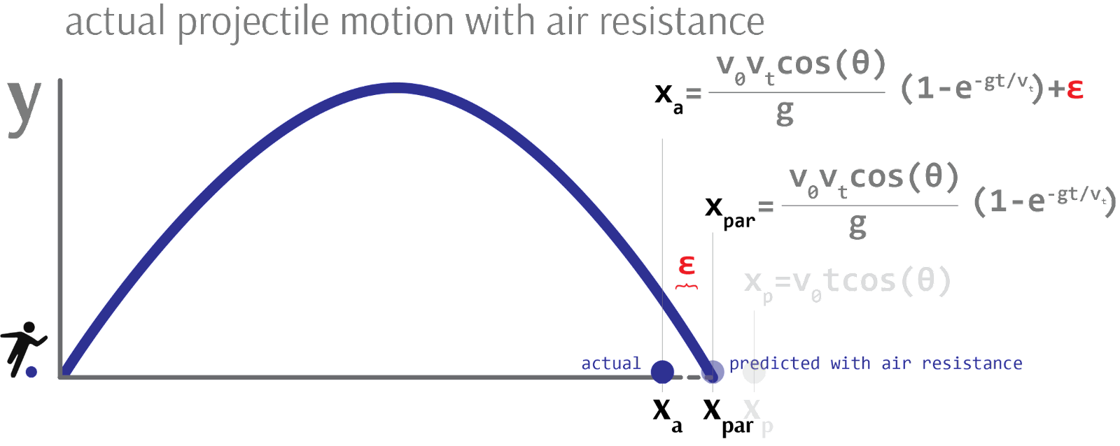
Image credit: Author’s own work
Is it possible then, in the far, far future, for us to actually possess complete knowledge of a system, to eradicate all randomness, to be Laplace’s demon? According to quantum physics, and specifically the Heisenberg uncertainty principle, the answer is no.
There exist properties of the universe, such as the simultaneous position and momentum of a particle, that are incontrovertibly unknowable, also known as quantum indeterminacy. The uncertainty principle therefore represents the fundamental limit on what humans can ever know and explain about the world.
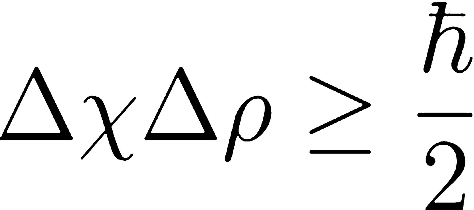
Image credit: Author’s own work
A practical example of model accuracy #
Returning to the notion of accuracy, let’s investigate an example using the infamous Norman door. A Norman door is a door which, by virtue of its design, is utterly ambiguous as to whether it should be pushed or pulled to open.
 Image credit: Author’s own work
We could develop a model of the door’s operation using many description languages:
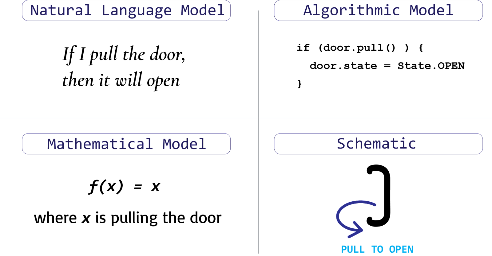
Image credit: Author’s own work
To test these theoretical models empirically, we must employ a statistical model and observe real-world outcomes.
We perform our first trial: we pull the door, but it does not budge. Here, our model predicted the door would open, but it stayed shut. Our first error. We pull again, and the door still does not open. Second error. Perhaps we are supposed to push, not pull, this door? At this point, our model successfully explains none of what we observe in the real world - it explains 0% of the observed outcomes and leaves 100% unexplained. For good measure, we pull once more - this time a good bit harder - and the door finally rips open. Our model has successfully predicted 1 out of 3 outcomes, leaving us with a final accuracy of 33%.
Model development and feature selection #
A model will be more or less accurate in describing the world depending on the components used. Some components are better than others. For example, omitting the engine when describing the operation of a modern vehicle would be a glaring oversight. Referencing an early 20th-century engine would be less accurate than a late 20th-century one, which too would be less accurate than one developed last year. The components we choose to include in a model and how we describe them therefore has implications for how accurate the model is.
In data analysis, this means that choosing to summarize our data using an arithmetic mean or geometric mean or harmonic mean has a material effect on the accuracy of our model. The decision to measure user engagement on a website using click activity versus days-on-platform is not arbitrary: only one of these (or some combination of them) will produce the most accurate model. In machine learning, this process of swapping in and out various components to maximize model fit is called feature engineering.
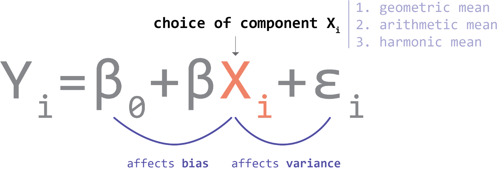
Image credit: Author’s own work
On inferential versus predictive statistics #
Before moving forward, I should clarify that model fit can be defined in two ways: an inferential way and a predictive way. Traditional statistics performs inference while more modern data science techniques perform prediction[0].
Traditional statistics attempts to infer structural models of the data - that is, the coefficients you see above - by observing data generated by a system (or a “data generating process”). The problem with this approach is twofold.
First, we often care more about how well the structural model predicts new data, as opposed to just having knowledge of the model’s coefficients when retrodicting historical data. Second, it is not hard to develop a structural model with a 100% fit to historical data. For example, if your model is “pull door once and it will stay shut, a second time still shut, but the third time it will open”, you will have a model with 100% accuracy, but also one which is overfit to historical data. The model’s performance on new data, known as out-of-sample fit, would be quite poor.
For these reasons, statistics evolved into data science, which focuses more on prediction. Many machine learning models do not attempt to build comprehensible structural models at all: to us humans, these models operate as impenetrable black boxes. The only thing that matters to them, very much by any means necessary, is that they maximize out-of-sample fit (or “cross-validation scores”): how well do they predict new data?
Nevertheless, despite their differences, both conventional statistical models and machine learning models develop models of the world to generate testable predictions and maximize accuracy.
--
[0] To be clear, statistics has always included a predictive component; indeed, machine learning is a subdiscipline of statistics. However, while “traditional statistics” tends to emphasize inference over prediction, machine learning exclusively studies prediction.