What does it mean for data to be “precise”? (Part 4)
(This post is part of a series on working with data from start to finish.)
The final aspect of measurement is precision. Precision is typically defined as the ability of an instrument to give identical values from measurements performed under identical conditions. While this would appear to be logically inevitable, it tends not to be the case in practice. In other words, measurements performed under ostensibly identical conditions yield different results.
Precision is measured in units of standard deviation, which refers to the degree of dispersion amongst measured results. If all measurements cluster around a single value, they are considered precise; if instead they scatter, they are considered imprecise.
This is conventionally taught using the metaphor of a bull’s eye: values close together are precise, whether or not they are actually close to the center of the bull’s eye (accurate). This bears repeating: precision has nothing to do with what we are actually trying to measure, and everything to do with the instrument itself.
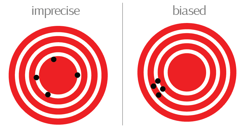
Image credit: Author’s own work
Returning to the marbles example in the prior post, let’s say we enroll more friends into our experiment over the subsequent days to count the number of marbles on the table. We might observe a distribution of estimates that looks like the following:
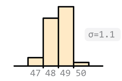 Image credit: Author’s own work
Precision refers strictly to the standard deviation of such a distribution and says nothing about the true number of marbles on the table (that is, the “population mean”).
The ISO definition of precision #
The sample’s distribution is narrow, but it could be even narrower - that is, more precise. To achieve this, we would ensure that measurements are conducted under increasingly controlled, and therefore identical, conditions. For example, one uncontrolled variable is that we are using many different people, or “operators”, to perform measurements rather than just a single one. Controlling this factor would increase our precision. In addition, we may want to ensure that all measurements are performed one after the other, rather than over the course of several days. This too will increase our precision. In fact, ISO identifies five such “repeatability conditions” that should be controlled in order to maximize precision of a measurement:
- the operator;
- the equipment used;
- the calibration of the equipment;
- the environment (temperature, humidity, air pollution, etc.);
- the time elapsed between measurements;
(ISO 5725-1:1994, 0.3)
If we were to ensure the same exact operator, the same equipment used, the same equipment calibration, the same environment and a short interval between measurements, we would expect to get the same results. And yet, in practice, we still do not! We can attribute this to “unavoidable random errors inherent in every measurement procedure,” ISO writes. “The factors that influence the outcome of a measurement cannot all be completely controlled” (ISO 5725-1:1994, 3.02).
Imprecision as unexplained variance #
Precision therefore represents the unknown, unexplained, “random” variability remaining in our measurements even after we control for all known, explainable, “systematic” sources of variability. It follows that the more sources of variability we are able to know, control and hold constant, the less unknown variability will remain, and thus the more precise our measurements will become.
Imprecision (random error), arising from factors we do not know about and cannot control, and incorrectness (bias), arising from factors that we do know about but do not control, together compose our “total displacement from the true value” (ISO 5725-1:1994, 0,6), or total error. In a statistical model, incorrectness refers to the alpha term (y-intercept), our deterministic displacement from the true value, while precision refers to the error term, our non-deterministic displacement arising from our inability to hold all conditions constant.
In plain terms, systematic error refers to the things you can control, but don’t, while random error to those you can’t even control for.
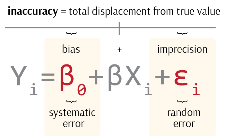
Image credit: Author’s own work
Let’s take another example. You step on a scale and measure your weight five times consecutively: 180 lbs, 182 lbs, 183 lbs, 181 lbs and 184 lbs. The mean weight is 182 lbs and its standard deviation is 1.6 lbs. Under such circumstances, we assume that very little about the conditions of the experiment have changed from measurement to measurement: same operator, same equipment, same calibration, same environment and little time elapsed. We cannot therefore attribute any of observed variation to those sources of variation, which would constitute bias, so what remains must reflect the scale’s inherent measuring imprecision of 1.6 standard deviations.
On the other hand, let’s imagine you performed those five measurements of the course of a week instead of a single day: 180 lbs on Monday, 182 lbs on Tuesday, 183 lbs on Wednesday, 181 lbs on Thursday, and 184 lbs on Friday. The statistics are the same: a mean of 182 and standard deviation of 1.6. However, the experiment conditions are not. Because we potentially allowed many known sources of variation to vary - the scale might have become uncalibrated between repeated use, the time between measurements has grown - we cannot confidently state what remains as unknown sources of variation. First, we’d have to control the known sources of variation!
In the example above, what is our actual weight? Well, we don’t know because we don’t know how imprecise the scale is to begin with. Did our weight truly vary over the week, or was this simply a reflection of the scale’s inherent imprecision? When we do not know an instrument’s baseline level of precision, we cannot disambiguate true changes in what we are measuring from routine statistical noise. The solution, according to ISO, is simple: always evaluate the precision of your instruments first before conducting any assessments of correctness (ISO 5725-1:1994, 4.12).
Precision as “close enough” #
Precision, from a practical point of view, is often referred to as “close enough”. Two measured values are often considered effectively equal if their difference falls within the range of an instrument’s known precision.
For example, imagine you are attempting to calculate the number of monthly active users on a popular social media website. There are many nuances that can make this a rather fraught exercise: you must exclude duplicate accounts, inactive accounts, deleted accounts, test accounts, bot accounts, spam accounts and so on. If different “operators” are to measure the amount of active users in a given month, it is unlikely they will do so in the same exact way. This frequently gives rise to conflicting calculations, an exasperating and all-too-familiar experience for executive teams who want a simple, reliable and unchanging number.
To the extent that all of these factors can be known and controlled for, there will be no variation in the reported user count. To the extent that any factor is known but not adequately controlled for, it will constitute bias, such as the bias of failing to exclude bot accounts from the total count. And to the extent that even after controlling for every factor we can think of - we use the same code, same data, same operator and so on - and there still remains unexplained variation in the total user count, we will tolerate it and call it imprecision.
If repeated calculations return user counts of “plus or minus” 50 users, which is the “typical” amount of variation we are unable to explain, we will ascribe it to the natural imprecision of our calculation methodology. If, on the other hand, subsequent calculations return differing counts of several thousand users, beyond our expected degree of imprecision, we will instead suspect a calculation error (that is, bias).
Therefore, differences greater than our level of imprecision are considered errors, whereas differences less than it are considered “close enough”.
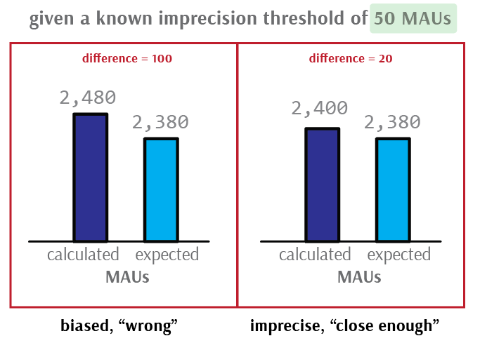
Image credit: Author’s own work
Precision and the history of science #
One might wonder why we settle for any unexplained variation at all. Surely if there exists variation we cannot explain, we ought to look harder to explain it. Indeed, much of the empirical sciences is devoted to such high-precision research. In order to maximize precision, we must control every possible condition of an experiment, thereby allowing us to vary only the variable we are interested in and measure its effect.
This approach perhaps found its most fervent practitioner in the French chemist Henri Victor Regnault, who emphatically declared “an instrument that gave varying values for one situation could not be trusted, since at least some of its indications had to be incorrect” (Chang 77). In other words, imprecise instruments were inaccurate instruments. Regnault believed that by designing exceptionally well-controlled experiments, one could eradicate imprecision, thereby producing truly accurate measuring instruments.
As chronicled by Hasok Chang in his masterful history of thermodynamics, Inventing Temperature, Regnault painstakingly developed exactly such experiments around the boiling temperature of water. Regnault resolved to discover the conditions under which water boiled at 100°C, as well those under which it “superheated” (did not boil) above 100°C. In doing so, Regnault reformulated what began as an accuracy question of “does water boil at 100°C?” into a precision question of “under what conditions does water boil at 100°C?” - and conclusively answer it. Through his pioneering research, Regnault demonstrated that questions of precision regarding our instruments must always precede questions of accuracy regarding the thing we are ultimately interested in.