The data pipeline: A practical, end-to-end example of processing data (Part 3)

This post comprises Part 3 of a 3-part series on data science in name, theory and practice.

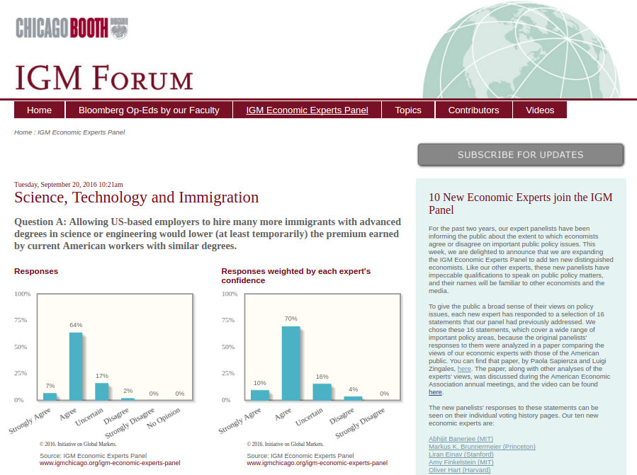
In Part 2 of this series, I discussed a systematic process for making sense out of data, without which it is easy to fall into the trap of drawing unactionable - or worse - unreliable conclusions. With the framework established, the goal of this post is to then walk through some of the code (in Python) required to implement it. I’ll use the IGM Economic Experts Panel dataset, which catalogs the responses of dozens of economists on public policy issues - you can see the results of my analysis here.

Below this initial landing survey are links to all the other surveys:

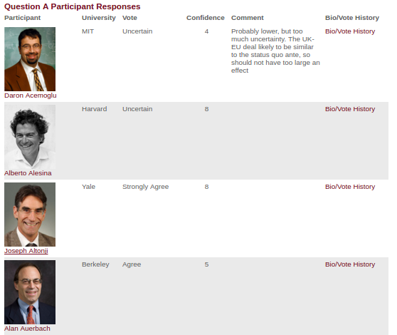
It’s within these surveys (i.e. each link) that I find the actual data tables listing each economist, their vote, their confidence and any comments they have.

So the roadmap is: scrape the homepage for the links to each survey, then scrape the response tables from each survey.

Now, how do I get the links to each survey? Ideally, all the links follow the same pattern. To check this, I inspect the DOM by right clicking on the link in Chrome and selecting “Inspect” (you can also view source with CTRL+U or F12). A frame will pop up that looks like this:

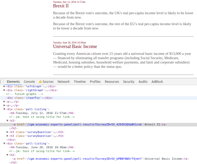
Here I see a pretty discernible pattern: each link is denoted by the <a> tag, nested within a header tag, wrapped in a <div> with an attribute of class=poll-listing (I end up using a slightly different pattern in the code). It’s good practice to isolate with a unique pattern - after all, there may be links within header tags whose wrapping <div>s do not have the poll-listing class.

Now that I know what to look for, I can write the code. Logically, I want to traverse the DOM and store each link in a collection (eg. list, tuple, dictionary).

domain = 'http://www.igmchicago.org'
response = requests.get(domain + '/igm-economic-experts-panel')
soup = BeautifulSoup(response.text, 'lxml')
polls = soup.findAll('div', {'class': 'poll-listing'})
topics = {}
for poll in polls:
    topic = poll.find('h2').get_text()
    handle = poll.find('h3', {'class': 'surveyQuestion'}).a['href']
    topics[topic] = handle

I use requests to pull the DOM of the webpage, http://www.igmchicago.org/igm-economic-experts-panel. Next, I parse the DOM using BeautifulSoup - essentially this gives me a shortcut to isolating certain elements (eg. links, tables, etc.), without which I’d have to structure myself. Using my BeautifulSoup object (in this case, the soup variable), I isolate all the <div> elements whose class attribute equals poll-listing. However, so far .findAll() has only given me an iterable ResultSet object, not the actual links I’m looking for. Therefore, I iterate over each Tag object (the poll variable) and use poll.find('h3', {'class': 'surveyQuestion'}).a['href'] to get the hyperlink as a string. I then store the link in the topics dictionary. Naturally, when using a new and unfamiliar package, I check the documentation religiously to understand all the methods which can make my job easier.

So after all that, I have the the links in a dictionary. Now I can iterate over each link, and for each page, scrape the tables on those pages. The resulting code is similar:

data = []
for topic, handle in topics.items():
    print(handle)
    response = requests.get(domain + handle)
    soup = BeautifulSoup(response.text, 'lxml')
    survey_questions = list('ABCD')[:len(soup.findAll('h3', {'class': 'surveyQuestion'}))]
    survey_date = soup.find('h6').get_text()
    tables = soup.findAll('table', {'class': 'responseDetail'})

First, I declare a data list object because pandas (the package for data tables) accepts data most easily as a list of dictionaries. Each element in the list is a row, and for each element, the dictionary’s keys represent the columns. As I scrape each row from the tables, I put each cell into a dictionary, and each dictionary is appended to the data list.

So given the list of links for each particular survey, I again use requests to pull their webpages, then BeautifulSoup to isolate the parts I need - in this case the <table> elements. (The line with list(‘ABCD’) basically says: assign a letter to each individual survey because the poll page can include one or multiple surveys).

Now for the next part of the code - what do I do with these tables?

for survey_question, table in zip(survey_questions, tables):
    rows = table.findAll('tr')#, {'class': 'parent-row'})
    for row in rows:
        if row.get('class') == ['parent-row']:
            cells = row.findAll('td')
            response = cells[2].get_text().strip()
            confidence = cells[3].get_text().strip()
            comment = cells[4].get_text().strip()
            tmp_data = {
                'survey_date': dtutil.parse(survey_date),
                'topic_name': topic,
                'topic_url': domain + handle,
                'survey_question': survey_question,
                'economist_name': cells[0].get_text().strip(),
                'economist_url':  domain + cells[0].a['href'],
                'economist_headshot': domain + cells[0].img['src'],
                'institution': cells[1].get_text().strip(),
                'response': response,
                'confidence': confidence,
                'comment': comment,
            }
            
        data += [tmp_data]

The first line essentially iterates over each table on the webpage, with a slight adjustment of tying the assigned letter to its respective table. Now, for each table, I need to pull all the rows (<tr> tags). For each row, pull (from left-to-right) the data in each cell (<td> tags). Retrieve and clean the actual text data from each cell (.get_text()), then put it in a dictionary with some sensible column names. Finally, append the dictionary (row) to the data list. Again, for some perspective, the data list will contain rows from every table on every poll webpage, so it’s important to make each row unique by including columns for the survey question (eg. A, B, etc.) and poll URL.

At last, I’ve scraped the data from all of the surveys! The last scraping step is to temporarily store the data in a more amenable format:

col_order = ['survey_date', 'topic_name', 'topic_url', 'survey_question', 'economist_name', 'economist_url', 'economist_headshot', 'institution', 'response', 'confidence', 'comment']
df = pd.DataFrame(data, columns=col_order)

For most datasets, you can persist this data (ie. a permanent format on disk, not just RAM) in a Python-specific pickle file or .csv:

df.to_pickle(os.path.join(os.path.dirname(__file__), 'igmchicago.pkl')

However, for some datasets, you’ll want use a relational database.

Storage #

pandas makes it easy to dump a dataframe into SQL, without which you’d have to use raw SQL (ie. building the schema and inserting the data) - a much more painful process. 

import sqlalchemy
engine = sqlalchemy.create_engine('sqlite:///igmchicago.db')
df.to_sql('igmchicago', engine, index=False, if_exists='replace')

Once your data is in a database, you can run plain-old SQL on it. For example, which economists have average confidence levels higher than the average for their institution?

cnxn = engine.connect()
r = cnxn.execute("""
  WITH igm AS (
    SELECT economist_name, institution, AVG(confidence) AS avg_conf
    FROM igmchicago
    GROUP BY economist_name, institution
  )
  SELECT * FROM igm i
  WHERE avg_conf >
    (SELECT AVG(avg_conf) FROM igm g WHERE i.institution = g.institution)
  ORDER BY institution, avg_conf
  """)
r.fetchall()

While I have a strong preference for fast, simple data manipulation in pandas, SQL is an absolute must for any data/BI analyst.

Exploratory Data Analysis #

After persisting the data, I need to understand what’s in it. What are the range of categorical variables and what do they indicate? Do some categories mean the same thing? Are there null values? How many rows are there and how many would I expect? I virtually always use the following commands to quickly get a sense of the data:

df.columns
df.shape
df.describe()
df.info()
any(df.duplicated())
df.head()
df.tail()
df['institution'].value_counts().plot(kind='bar')

EDA will accomplish two things: (1) you will learn the correct interpretation of your data and (2) you will identify some (presumably not all) errors in the data which need to be corrected. In this case, I noticed a couple of issues with my original scraped data.

Data Cleaning #

First, I saw that virtually all the recently added economists had very low survey response rates. I checked into the original data and noticed that although these economists were given the opportunity to retroactively respond to surveys, these responses were included as a second row, not the initial row which I scraped. 

So I had to go back through my scraping code and rescrape the second row if it had data in it. After doing this, I confirmed that the discrepancy in survey response rates between newly added economists and all other economists was removed. Success!

Second, all comments were stored as a string, even if they were blank (ie. an empty string: “”). The summary statistics therefore would lead one to believe that every economist always left a comment, which was obviously untrue. As a result these empty strings needed to be recoded as null values.

Finally, I decided that adding the sex of economists would be useful and coding the response categories as numeric values would facilitate aggregation.

# Correct response types
df.loc[df['response'].str.contains(r'did not', case=False) | df['response'].str.contains(r'---'), 'response'] = np.nan

# Convert empty string comments into null types
df['comment'] = df['comment'].replace(r'^$', np.nan, regex=True)

# Assign sex variable to economists
sex = pd.read_csv(os.path.join(os.path.dirname(__file__), 'economist_sex_mapping.csv'), index_col='economist_name')
df['sex'] = df['economist_name'].map(sex['sex'])

# Assign response categories to numerical values    
certainty_mapping = {
    'Strongly Disagree': -2, 
    'Disagree': -1,
    'Uncertain': 0,
    'No opinion': 0,
    'Agree': 1,
    'Strongly Agree': 2,
}
df = df.assign(response_int = lambda x: x['response'].map(certainty_mapping))

Data Analysis #

Data analysis is often the meat of any data-driven project: you’ve gathered, stored, understood and validated the data, now how can you use it to answer business or research questions?

I did not thoroughly analyze this dataset, though there is a lot I could do. I could run a regression with dummy variables and see if sex was associated with more or less confidence in responses. I could find the average confidence by institution, or tabulate an economist’s confidence level over time. In many cases, I don’t need more than intermediate statistics. A lot of insight can be gained by simply looking at any metric by a dimension (eg. region, sales channel, etc.), over time, or as a proportion of the total. 

Here are some quick summary statistics I ran with pandas. 

facet_labels = ['economist_name', 'institution', 'sex']
facets = df.groupby(facet_labels).first().reset_index()[facet_labels]

# Summary statistics
len(df.groupby('topic_name')) # 132 topics
len(df.groupby(['topic_name', 'survey_question'])) # 195 survey questions
len(facets['economist_name'].unique()) # 51 economists
facets.groupby('sex').size() # 11 female, 40 male
facets.groupby('institution').size().sort_values(ascending=False)

Data Visualization #

I am a strong advocate of visualizing everything. Your audience will rarely be statisticians or analysts - often, they are decision-makers who simply need to know the next step and want a quick way of seeing the data-driven evidence. Not only that but visualization will quickly show you if your results seem counter-intuitive, allowing you the chance to review your data and analyses before presenting them.

Unlike R, which has the powerful and intuitive ggplot2, Python does not feature as robust plotting libraries. The most popular packages I have seen are seaborn, ggplot (ported from R), bokeh (displays in the browser), and the low-level matplotlib. In my opinion, none of these are as mature as ggplot2 due to either bugs or lack of features. While working on this project, I toyed with each library but eventually settled on matplotlib to visualize exactly what I needed - of course, at the cost of concise code and readability. 

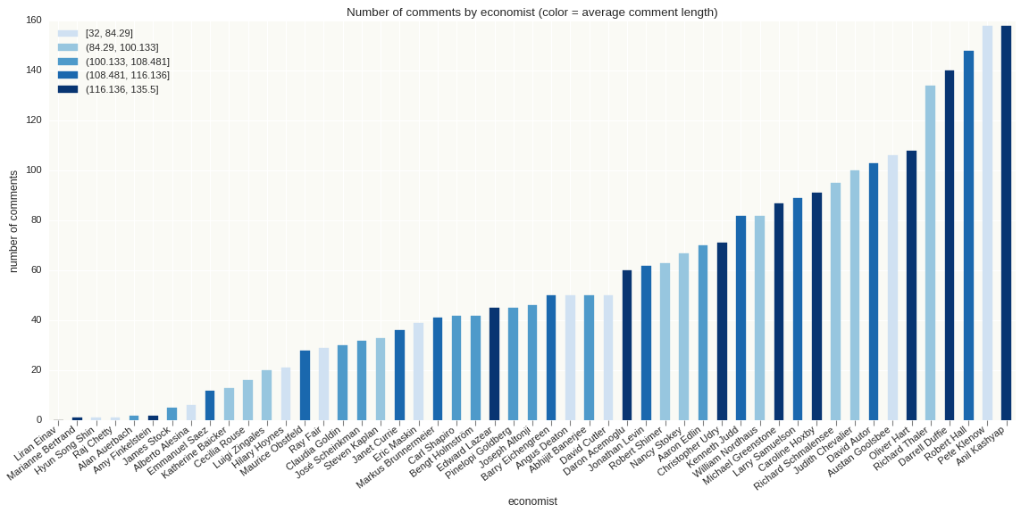
For the sake of brevity, I decided not to include the code to visualize the data here, but you can view the graphs here and the code on GitHub.

That wraps up a high-level overview of implementing the data pipeline from start to finish. I strongly believe that once you understand the main steps in the process, most analytical projects become feasible. If you need new data, or have to clean data, or need to store and query large amounts of data, or visualize data, all you need is an understanding of these basic principles.

Hope you enjoyed reading! This post concludes the 3-part series on data science in name, theory and practice.

Full code for this project can be found on GitHub.